Infinite Impulse Response (IIR) digital filters

Break from statistics. I want to talk about digital signal processing again. So I talked about FIR filters before, let’s talk about IIR filters. Like how to recognize them, analysis, maybe things like direct form type I and II later, and then at least simpler design like Butterworth IIR filter design, and a mention of the transforms to go from analog to digital domain.

So what is an infinite impulse response filter? Well, it’s a filter such that a resulting signal from passing something through doesn’t really ever die off completely. Lemme bring back the easy example I used in my FIR filter post.

Let’s say our input is a Kronecker delta such that and everywhere else it’s just nothing. When , . At the next time step, . And the next time step, . And so you can see with every time step, our resulting signal is getting smaller, and it does converge to 0, but it just keeps going and going.

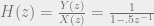
So how can we find the impulse response? We can use the z-transform like we did for FIR filters.

We know our impulse response is output over input, so

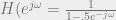
And of course, if the region of convergence for our z-transform includes the unit circle, we can find the discrete-time Fourier transform simply by replacing z with ,

And just like that, we have our impulse response for our IIR filter. Yeah, this one is kind of trivial but it’s just for teaching purposes.

So how do we know if our IIR filter is stable? With FIR filters, we knew it was going to be stable no matter what. The output signal would end, assuming input was bounded and finite already. If we look at our IIR filter Z-transform, given a more complex one, we can see that with a polynomial on top and bottom, we will have zeros such that some complex values of z will make the filter equal to 0, and we will have some poles such that some values of z make the filter shoot to infinity. The general rule is that given a CAUSAL filter, like one that doesn’t somehow go backward in time, if the poles are inside of the unit circle, the unit circle is included in the region of convergence and our filter is stable. So that’s cool. I mean, if zeros are inside of the unit circle, then we also have less of a phase mess-up problem too, but that’s less of a problem than unstable filters.

So what are the pros and cons of IIR filters? In a lot of situations, IIR filters can get the desired filter response wanted using significantly fewer filter coefficients than FIR filters. In many situations, IIR filters that have been turned into biquads or filter banks, basically split into packs of smaller IIR filters, are pretty computationally efficient if you don’t have the luxury of doing zero-padded FFTs for FIR filters.

The downsides? IIR filters tend to be pretty sensitive to limitations of computer numbers. If the machine precision isn’t good enough, the actual filter behavior may not function as planned. Even if the filter acts like you’d expect at the beginning, the numerical precision thing leads into a feedback problem, say the filter behavior EVENTUALLY turns into garbage because of numerical limitations. This can be solved with a zeroing of values, basically resetting the filter, at some point, but that may mean tossing out information. Additionally, IIR filters aren’t conveniently linear phase or zero-phase like FIR counterparts can be designed, so if you need real-time signal processing, get ready to have some phase changes. These can be minimized if the filter is designed such that zeros are within the unit circle. Additionally, if the real-time requirement isn’t there, you can do a forward-backward filter process to have a zero-phase filter by simply doing the filter, and then using a time-reversed version of the filter.

I’m too lazy to fire up python or matlab, but you can use the examples from the FIR filter to do analysis of IIR filters. freqz(b,a,n) in both python and matlab are designed such that b is a vector of coefficients in the numerator of H(z), a is a vector of coefficients in the denominator of H(z), and n is some number of samples that basically lets you set a resolution to look at. Note that for FIR filters, we set a = 1 because we don’t have any denominator to H(z) to worry about.

Generating random samples pt. 3 – Metropolis-Hastings algorithm

So last time I talked about rejection sampling for generating random samples of a specific distribution, starting from another distribution. We talked about what made it suck, and really, if you are going to do rejection sampling, you might as well head straight to Metropolis-Hastings, it’s basically an improved version with no downsides when compared to rejection sampling.

So the Metropolis-Hastings algorithm is another Monte Carlo method of generating samples, and really, it’s basically rejection sampling with a minor change. So I’ll go over the gist of it, and then point out the change, and why Metropolis-Hastings even works.
The algorithm is as follows.
Given a target PDF of and SYMMETRIC densities of (symmetric meaning ) that we are drawing samples from, where g is conditioned on the previous sample we had accepted,
1. Get a sample x from , and a sample from a uniform random variable between 0 and 1, i.e. , which we’ll MIGHT be using to make our decision whether or not to keep or reject the new sample.
2. Check if we keep the sample; if , such that the PDF of the new sample is larger than the previous one, we keep our new sample straight up. Otherwise, we need to do a check against our uniformly distributed value; if our uniformly distributed random sample , then we keep the new sample x. Otherwise, we reject x.
3. If we kept the previous sample, is replaced with the x we just got. Go back to step 1 and keep doing it until we have enough values.

A common example of is a Gaussian distribution with a mean of . Then the resulting process will be something of a random walk, which very nicely lines up with the Markov chain proof of correctness for this algorithm. I’M not going to prove it is right, but there certainly is proof, this process is pretty old.

So what’s the big deal? We changed our criterion for keeping samples. On inspection, you’ll note that we don’t need a dumb scaling constant anymore, and assuming we chose nice source and target distributions to work with, our acceptance rates will be much nicer than before.

But you might think, hey, if we accept more stuff like this, how can we guarantee Metropolis-Hastings even gives us samples pertaining to our target distribution?

In truth, the Metropolis-Hastings algorithm is loosely construction a Markov chain system like the ones we’ve suggested before. What we are doing is moving from state-to-state as we accept samples, and our Markov chain is constructed in such a way such that the stationary distribution of the Markov chain will be the target distribution! Of course, for a target PDF, since it’s a continuous function, this is not intuitive to see, but working with a discrete PMF, say, something trivial like simulating a fair 6-sided die by choosing a conditional such that each roll is biased (evenly, like the PMF is simply being shifted over a single value at a time from 1 to 6) more towards the number last rolled, it’s very possible to construct the transition matrix and see that the end stationary distribution of the system will be that of a fair die. An example would be a transition matrix like this…

Even though the die is a biased turd, if we generated dice rolls over time with this transition matrix, the stationary distribution in the end would be a nice uniform fair die.

So what are the downsides to this? Well, samples tend to be correlated with their neighboring samples, so if you want uncorrelated samples, you sort of have to give the samples a good shuffle. Additionally, the first bunch of samples generated clearly won’t be distributed as we’d want because the Markov chain hasn’t had time to hit a stationary distribution, so expect to have a burn-in period of running the algorithm, throwing things away, and then getting samples to use.

Hell, I’m lazy, you can fix my previous function to work with Metropolis-Hastings if you really want, the change is trivial and my previous function wasn’t great anyways. I wrote it in maybe a couple minutes.

Next time, if I get the chance, I will discuss Gibbs sampling and wrap up what I want to say on generating samples of a target distribution.

Generating random samples pt. 2 – rejection sampling

So I covered basic inverse transform method of generating samples of a specific distribution, and all that required was basically knowing the CDF and inverting the function, followed by feeding it uniformly distribution samples from 0 to 1 and that was that. However, some distributions are difficult or nearly impossible to invert analytically, so… where does that leave us?

So rejection sampling, also known as the acceptance-rejection method, is a Monte-Carlo method that allows us to simulate generation of samples of basically any probability density. The idea behind it is that we can sample a random variable by sampling uniformly underneath the graph of a density function.

The gist of the algorithm is as follows:
Given a target PDF of , a normalization constant M that effectively adjusts frequency of rejection when increased, and a density of that we are drawing samples from,
1. Get a sample x from , and a sample from a uniform random variable between 0 and 1, i.e. , which we’ll be using to make our decision whether or not to keep or reject the new sample.
2. Check if we keep the sample; if our uniformly distributed random sample , then we keep x. Otherwise, we reject x.
3. Go back to step 1 and keep doing it until we have enough values.

You can see from the algorithm that increasing M would decrease the probability of retaining generated samples, but M additionally has to be set such that so that step 2 actually makes sense, avoiding violating axioms of probability.

An example written in Python is available below. Basically, it wants a function f_x passed in representing a 1D PDF of the target distribution we want. We are using Gaussian random variables for our drawn g_x function because the domain is infinite and we can fine-tune where we sort of want our concentration using the parameters. Then M and number of samples is up to the user, though if M proves to be too small, M is doubled and the function is called recursively in hopes that things will work out better next time.

import numpy as np

def rejection_sampling_1D( f_x, g_var, g_mean, M, num_samples ):
    ''' does rejection sampling using a Gaussian distribution as  the
    underlying density, given a target density function f_x and a number of
    samples we want generated.'''
    g_x = lambda x: 1/np.sqrt(2*np.pi*g_var)*np.exp(-(x-g_mean)**2/(2*g_var))
    good_samples = 0;
    # do shit until we have enough samples
    keepers = np.zeros(num_samples)
    while good_samples < num_samples:
        # generate a new sample using our underlying distribution
        new_samp = np.random.randn(1)*np.sqrt(g_var)+g_mean
        # generate a new uniform
        new_check = np.random.rand(1)
        # first, let's make sure M is big enough
        while f_x(new_samp)/g_x(new_samp)/M > 1:
            M = 2*M
            return rejection_sampling_1D( f_x, g_var, M, num_samples )
        # now let's check if our stuff actually works.
        if new_check >= f_x(new_samp)/g_x(new_samp)/M:
            keepers[good_samples] = new_samp
            good_samples = good_samples + 1
        else:
            continue
    return good_samples

So what’s wrong with this? The first major problem is that if distributions are chosen poorly, like if isn’t remotely related to , a lot of samples may be generated and tossed away, wasting computation cycles, or a lot of samples may be taken in a specific area, getting us a lot of unwanted samples. The former result is magnified immensely once we begin talking about multidimensional random vectors, running straight into the curse of dimensionality, where chances are corners and edges of our multidimensional density simply don’t get the coverage we were hoping for.

Next time, we will talk about Metropolis-Hastings method for generating random samples. It’s better than rejection sampling, and it also partially ties into our Markov Chain talks before, though I won’t get into that in too much detail. If I get a chance, I may also talk about Gibbs Sampling in a post afterwards.