On stationary distributions of discrete Markov Chains

I feel like I need to publish something quick, so I’ll just discuss stationary distributions for Markov Chains real quick before my orientation stuff at Cisco in California. I don’t necessarily know if I have time to make a post while I’m there.

We’ve discussed Markov Chains previously. Given a set of states, say n states such that where S is the set of all states we care about, we have a transition matrix that is n x n elements, say a matrix A like the following:

where the transition matrix entry is the probability of being AT state i, and moving to state j. REMEMBER THIS, because some books like to refer to it the other way around, like i is the target state and j is the previous state, and that changes our notation up entirely here.

For simplicity, you can assume our Markov Chain is time-invariant, meaning the probabilities in the transition matrix don’t change over time. I believe what we are discussing here will hold, but definitely not in a obvious and conveniently calculable way, like there’s going to be symbols and stuff, and potentially you’d probably have to prove that the markov chain remains positive recurrent over time, weird shit, let’s not get into that. Let’s assume we have a nice matrix full of constants that don’t change with each time step.

So say we have a starting distribution of what state we might be in, a row vector x such that . The subscript of X indicates which time step we’re talking about, and 0 is obvious the start. We can find the probability of being in whatever state at time step t by doing the following
so we have a row vector multiplied by our A transition matrix to get us another row vector with the changed probabilities of being at each state at whatever time step. So that’s cool, right? Very handy in terms of calculation. Assuming your transition matrix is legit, like the rows add up to 1 properly, then your X elements should also sum up to 1 all the time. You can prove this but it takes some work, just accept it for now.

So a stationary distribution is when we have some row vector Y such that , so when you multiply the row vector Y with the transition matrix, there is no change to the elements of Y, the probabilities remain the same. This stationary distribution typically comes up as a limiting distribution where . So yeah, if you want to brute force your way to a stationary distribution, you can calculate it on a computer by doing matrix multiplies over and over until hitting some convergence point.

But linear algebra people should recognize that Y here is actually a LEFT eigenvector! You can solve for this simply by solving for the (right) eigenvectors of , the transpose of the transition matrix, and finding the eigenvector associated with eigenvalue 1, and normalizing it such that it is a legit discrete probability vector. So there’s a clear relation of linear algebra to Markov chains.

Obviously, there has to be a catch to this bit, right? So there are three things that could happen with stationary Markov chains.
1. unique stationary distribution
2. multiple unique final distributions
3. oscillating/alternative final distributions

The uniqueness of the stationary distribution is only guaranteed iff the MC is positive-recurrent. What does that even mean? The simplest way to find it is by making sure each state is reachable at any time, i.e. they are all recurring states, and that the periodicity of each state going back to itself eventually has a greatest common factor of 1 (like there could be a state that goes back to itself potentially even 2 steps at the quickest, but somebody else could only do it in minimum 3 steps, then the GCF is 1). In linear algebra terms, this effectively guarantees the matrix is full rank, geometric multiplicity of eigenvalue 1 is 1 (there’s only 1 eigenvector associated with eigenvalue 1), and there’s no weird thing involving eigenvector -1.

How do 2 and 3 even occur then? 2, if you effectively have transient states, or just completely separable Markov chains you happened to put into the same matrix (like with 5 states, if states 1-3 communicated amongst themselves and 4,5 communicated only between themselves), you will end up with more than 1 stationary distribution at the end. In case 3, if there’s some periodicity going on, then clearly it’s possible that the Markov chain will have some alternating with each time step and not actually be stationary by the end, though it will have converged to a set of probability vectors. Generally, you may end up with a eigenvector for eigenvalue 1, and then an eigenvector for eigenvalue -1 that will represent the change in the distribution with every time step.

Linear classification using least-squares

Let’s talk about another application of least-squares in statistical learning applications. Say we have some data, and we want to separate them into groups. We have some data that we separate into training and validation sets that we know what groups they should be in. For data in an n-dimensional space (say, the data is defined by n coordinates, or in even simpler terms, has n features), we need to find hyperplanes of dimension n-1 that will SPLIT the space in half, where everything on one side is in one group, and everything on the other side of the hyperplane is in another (Intuitively, for our purposes, you can see 2D Euclidean space can be separated into two parts by a line, which is a 1 dimensional object, and a 3D euclidean space can be split by a plane, which is a 2D object).

So how do we find said hyperplane to divide up our space? The simplest way, and probably the most common way still just because it’s easy for a first-shot attempt at classification and linear regression, is to employ least-squares.

Let us say we have training data points of n dimensions, training points each designated at , for the ith index training point, jth coordinate . These training points belong to two classes, which we’ll classify as the -1 team and the 1 team. Since hyperplanes are represented most easily in equation , where where is a constant and is an n-dimensional vector of coefficients, our goal here is to solve for the a coefficients and the b constant.

So let’s arrange the problem thusly; we want our matrix for the least squares problem to contain our data points, such that

So we have our rows of data points stacked on top of each other, with a column of 1s representing a constant offset of b in our hyperplane equation. The b vector is obviously then just going to be a stack of -1s and 1s for whatever class each row data point is matched to.

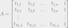
And then obviously since this is least squares, our resulting vector of coordinates is going to be

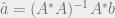
We have our hyperplane, now how do we do validation or classification of new data points? Recall that we classified our points using -1 and 1 teams. Adding a 1 to the tail of each data point like we did before to represent the constant b term in the hyperplane equation which we have in our coefficients, we can use our hyperplane equation’s left side, , and simply classify points depending if the result is negative or positive!

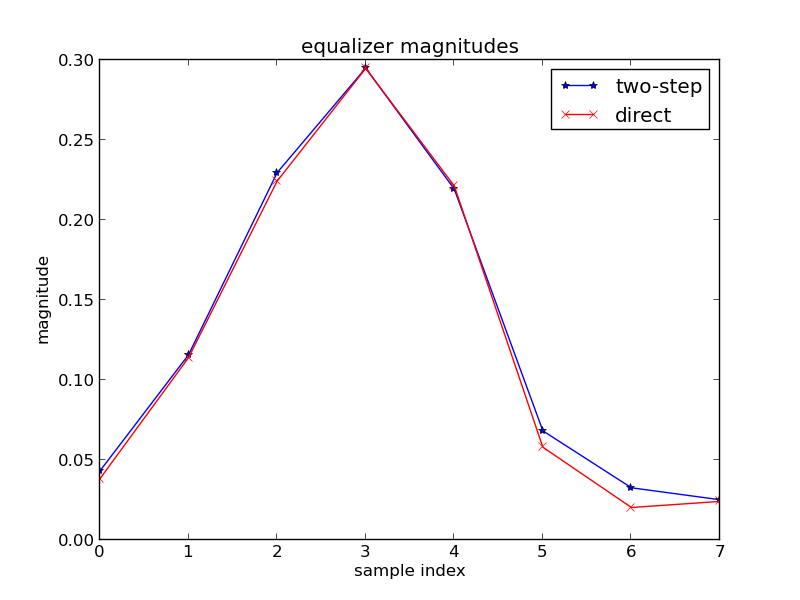
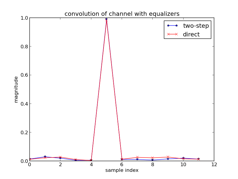
The MATLAB code below provides an example of a hyperplane separating two 2D Gaussian populations, and then trying to use that rule to classify data with a higher variance than we expected. A plot with training data points and the separating hyperplane is generated, and then a print out of percentage of correctly classified points is given at the end.

% generate 2 2D pops
ndim = 2;
pop_size = 20;
u1 = [4, 4];
u2 = [-2, -1];
covar_mat = 5.*eye(2);
pop1 = bsxfun( @plus, randn(pop_size, ndim)*chol(covar_mat), u1 );
pop2 = bsxfun( @plus, randn(pop_size, ndim)*chol(covar_mat), u2 );
figure;
plot( pop1(:,1), pop1(:,2), '*b' );
hold on;
plot( pop2(:,1), pop2(:,2), 'xr' );
% find the hyperplane that goes through the middle using least squares
A = [[pop1; pop2], ones(2*pop_size,1)];
b = [-1.*ones( pop_size, 1 ); 1.*ones(pop_size,1)];
coefs = lscov(A, b);
% plot the coefficient line using that learning data we generated
line_x = [-20; 20];
line_y =  (-coefs(end)-coefs(1).*line_x)./coefs(2);
plot( line_x, line_y, '-k' );
xlim( [-20, 20] );
ylim( [-20, 20] );
% now let's try to classify the new points we generate
covar_mat2 = 8.*eye(2);
new_pop1 = bsxfun( @plus, randn(pop_size, ndim)*chol(covar_mat2), u1 );
new_pop2 = bsxfun( @plus, randn(pop_size, ndim)*chol(covar_mat2), u2 );
combined_newpop = [new_pop1; new_pop2];
new_inds = randperm( (2*pop_size) );
actual_population = b(new_inds);
combined_newpop = combined_newpop( new_inds, : );
newpop_w_ones = [combined_newpop, ones(2*pop_size, 1)];
classify = sum( bsxfun( @times, newpop_w_ones, coefs(:)' ), 2);
classify(classify < 0) = -1;
classify(classify >= 0) = 1;
percent_correct = sum(classify == actual_population)./(2*pop_size)

So what’s wrong with this? The clearest problem is that this method really implies that groups are linearly separable, and a lot of times, it’s not that simple. This method also tends to allow outliers to have really heavy effects on the resulting lines, and generally does poorly for classification of more than 2 groups, no matter how you decide to handle the multiple group problem (1v1 hyperplanes or 1 vs everybody else hyperplanes, either way). Inherently, since linear least squares is optimal ML estimator for Gaussian populations, you are inherently assuming multivariable Gaussian distributed stuff, and even if it is, there’s somewhat of a disregard for prior information, say, covariance matrices or anything else that might help.

Since the follow up is natural and I really want to get this stuff nailed down for myself, next time we will talk about linear discriminant analysis, and then after that, quadratic discriminant analysis. I personally think of LDA and QDA as a more thorough treatment of the linear classification problem by stating assumption and taking in account parameters that may help us, plus QDA has the benefit of generating quadratic lines.

Using least-squares for channel estimation pt 2: Python implementation

So I talked about using least-squares to estimate a channel at the receiver of a communication system, given some known training sequence. Now I have code to put it into practice. The code will be posted below, but I’ll start with an explanation of what I have done first up here before delving into the details after the code.

So the code can be broken up as follows. First, I generate a channel of some random values. I generate some Rayleigh fading values using a Gaussian number generator (by the way, I make no claims as to how realistic or unrealistic this channel is, I’m just using it to prove that the estimation deal works. Realistic channels or even existing models for channels can be discussed some other time).

Next, I generate a pseudonoise training sequence of +1 and -1 values that I would send through my communication system. Realistically, I would use a Gold sequence, or a Barker sequence, some special binary sequence that guarantees good properties for synchronization purposes, but I just randomly generate a binary sequence here.

I apply the communication model we discussed before, where the received signal is , where h is our discretized channel, x is the sent signal, and v is additive white Gaussian noise.

Now the fun begins. I estimate the channel using least squares exactly as I had modeled in my previous post, creating a Toeplitz matrix using known training values and forming a “b” vector out of actually received values. I use this estimated channel to find an equalizer that best cancels it out by forming a Toeplitz matrix using the estimated channel, and having a Kronecker delta vector for the “b” vector. Finally, I form a Toeplitz matrix out of received values, form a “b” vector out of known training values, and solve for an equalizer directly. Two steps is definitely not better than one when there’s noise to be accounted for.

So here’s the code.

import numpy as np
import matplotlib.pyplot as plt
import scipy.linalg as la

# parameters go here
L = 5 #length of channel
Lf = 8 #length of equalizer
Nt = 22 #length of training sequence
noise_pwr = .01 #AWGN variance
nd = np.floor((L+Lf)/2.0)

# generate channel, random Rayleigh variables
h = np.random.randn(L) + 1j*np.random.randn(L)

# generate pseudonoise training sequence
t = np.random.randn(Nt)
t[t<0] = -1
t[t>=0] = 1

# apply our frequency selection comm model with AWGN
y = np.convolve(h, t) + np.sqrt(noise_pwr)*np.random.randn(L+Nt-1)

# estimate the channel
b = y[L-1:]
col = t[L-1:]
if b.size > col.size:
    append_zeros = b.size - col.size
    col = np.hstack( (col, np.zeros(append_zeros) ))
row = np.flipud(t[0:L])
A = la.toeplitz(col,row)
h_hat,_,_,_ = np.linalg.lstsq(A, b)

# find an equalizer
col = np.hstack( (h_hat, np.zeros(Lf-1)) )
row = np.hstack( (h_hat[0], np.zeros(Lf-1)) )
A = la.toeplitz(col, row)
b = np.zeros(h_hat.size + Lf - 1)
b[nd-1] = 1.0
f,_,_,_ = np.linalg.lstsq(A, b)

# now just solve directly for equalizer
row = np.flipud(y[:nd])
if row.size < Lf:
    row = np.hstack( (row, np.zeros(Lf-row.size)) )
elif row > Lf:
    row = row[:Lf]
b = t
col = y[nd-1:]
if col.size < t.size:
    col = np.hstack( (col,np.zeros(Nt-col.size)) )
elif col.size > t.size:
    col = col[:Nt]
A = la.toeplitz(col,row)
f_d,_,_,_ = np.linalg.lstsq(A,b)

# convolve with original channel to see how our equalizers are
res1 = np.convolve( h, f )
res2 = np.convolve( h, f_d )

# plot the results
plt.figure()
plt.plot( np.arange(h.size), np.abs(h), '-*b', label='actual')
plt.plot( np.arange(h_hat.size), np.abs(h_hat), '-xr',label='estimated')
plt.title( 'channel magnitudes' )
plt.xlabel( 'sample index' )
plt.ylabel( 'magnitude' )
plt.legend()
plt.savefig( 'ls_ch_est_1.png' )

plt.clf()
plt.plot( np.arange(f.size), np.abs(f), '-*b', label='two-step')
plt.plot( np.arange(f_d.size), np.abs(f_d), '-xr',label='direct')
plt.title( 'equalizer magnitudes' )
plt.xlabel( 'sample index' )
plt.ylabel( 'magnitude' )
plt.legend()
plt.savefig( 'ls_ch_est_2.png' )

plt.clf()
plt.plot( np.arange( res1.size), np.abs(res1), '-*b', label='two-step' )
plt.plot( np.arange( res2.size), np.abs(res2), '-xr', label='direct' )
plt.title( 'convolution of channel with equalizers' )
plt.xlabel( 'sample index' )
plt.ylabel( 'magnitude' )
plt.legend()
plt.savefig( 'ls_ch_est_3.png' )

Let’s talk about some of the nuances of why any of this works. All three of the least squares problems are developed such that every problem is overdetermined. I’m going to say again, do NOT do it with an underdetermined system, and if you have a square A matrix, this probably isn’t going to work our well for you. Basically, choose a training sequence that is long enough, and an equalizer that is at least as long as the channel, and shorter than the training sequence by some amount, and you’re probably golden. Realistically, this probably won’t be a problem if you use a preset sequence for channel estimation, like concatenated Barker codes or something.

There are some places where I have if statements for appending zeros or shortening vectors before forming the Toeplitz matrix. Frankly, the matrix created needs to fit the parameters you have on hand, and there may be times where you need to fill in zeros because there’s nothing left in your convolution to express in the linear system.

The number of sequences I choose to delay here is the recommended rule-of-thumb by Dr. John Cioffi at Stanford, like I discussed before. If you change the value to be one more or one less, I’m pretty sure you can get some results that give you a less-than-perfect Kronecker delta for the final plot of channel convolved with equalizer.

Solving for an equalizer in two steps makes the problem easier to visualize, but in general will obtain worse (maybe not by much) results than the direct equalizer solve. The noise effects tend to get worse using two operations.

An example set of plots generated is given below. Remember that the channel and stuff shown here are just magnitudes, so don’t try to visually convolve them, that’s just going to make things confusing.

Interesting bit about Least-Squares

Let’s talk about the least-square solution to linear systems of equations. Let’s say we have the problem

where A is an m-by-n matrix (m rows, n columns), x is an n-element vector, and b is an m-element vector. This is just a standard form of a linear algebra problem. Let’s also assume A is full-rank.

Now’s let’s say , or A is a tall matrix. We call A an overdetermined matrix. Simply put, there are way too many unique linear equations to solve for a unique x vector answer. So what do we do? We can use least-squares formulation of the problem to get some sort of an acceptable answer. If we multiply by sides of the equation by the Hermitian transpose of A, we get

So we have a least-squares solution for x. For people well-versed in linear algebra concepts, this is essentially the projection of the vector b on the subspace spanned by matrix A. But generally speaking, most people don’t care about that. Why is least-squares good for this case then? The least squares solution we obtained here minimizes the function

So the vector x minimizes the error for the equation. We cannot obtain an exact x for our overdetermined system, but this is our best shot, in terms of this squared error measure.

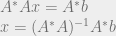
But wait! If , or A is a fat matrix, A is then an underdetermined matrix, and we have a large solution space. The vector x could be a whole number of things! What’s neat about least squares is that we can still use it here for a similar purpose.

So why is this useful? The vector x here is actually the solution to the system with the smallest norm, so is minimized. There are places in optimization or control theory where we want the minimum energy vectors for controllability or stability, so the underdetermined least-squares problem is useful as well.