Expectation-Maximization Algorithm. In general.

Previously, we discussed the maximum a posteriori estimator and the maximum likelihood estimator. We gathered that using given data, we can make use of Bayes’ theorem and make a solid guess at parameters of a probability distribution, given the data we got and any prior knowledge. Even if we had no prior distribution, we could just get a solid guess thanks to MLE.

But let’s say the situation got a little more complicated. Last time, we discussed classification by linear discriminant analysis (LDA) and quadratic discriminant analysis (QDA), but those technically require us to have the parameters for the distributions of each class known ahead of time. So what if we need to guess that? Each class is going to have a distribution, and we have a bunch of data with no known classes, so how can we bridge the gap and not only classify our data but make a guess at the parameters of each class?

So the Expectation-Maximization algorithm gives us a method to basically try our best to get all the things we want to solve for above, landing at a possible local solution but maybe not the actual answer. Which is fine, we’re just making a guess. Sometimes that’s the best we can do.

Informally, what the algorithm entails is looping the E and M steps until convergence.
1. Expectation step: Using the prior from the previous step, find the expected value of the underlying variables we need in our setup; e.g. for classification, let’s classify the points by choosing the class we would expect each data point to be in, given our prior distributions from the previous step.
2. Maximization step: using the underlying variables we just solved for in the E step, use maximum likelihood estimators to find parameters for the distributions of whatever we’re looking for, e.g. for classification, the distribution of the classes.

In more formal math terms, lets say X is a vector of data, Z is the underlying variables we need, is the log likelihood function for parameters, given X and Z, and is a vector of parameters we want to solve for. Breaking the algorithm up into 2 steps like before,
1. Expectation step; calculate the expected value
2. Maximization step; calculate new

So how would we do this for our little Gaussian mixture model we wanted to classify in the previous post? We have m classes, n data points (for now, let’s assume n >> m, we have tons of data). Making guesses at our parameters initially for each class, we do EM by repeating the following 2 steps.
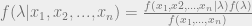
1. Expectation step: find which class a point belongs to using LDA or QDA classifiers from the previous post (the assumptions each one assumes applied here, so choose one and stick with it).
2. Maximization step: for each class, use the points associated with it to find the sample mean. For LDA, we find the sample covariance matrix using all points so this won’t change between iterations, but for QDA, we need to also find the sample covariance matrix for each class.

If we wanted to entire ignore covariance in this calculation, you could actually see that k-means using a simple distance measure to decide on classes for the expectation step is basically an expectation maximization algorithm! Additionally, you can see that Baum-Welch is a variant of this for Hidden Markov Models where during our expectation step, we guess what states our system is in, and then use that to make a guess at our observation and state transition matrices.

Couple things: clearly, EM is a very general idea; the algorithm details need to be changed depending on the problem, i.e. things aren’t just Gaussian all the time, we need to adjust EM to suit our problems. EM algorithm tends to fall into a local solution but not necessarily the solution you want, and of course this changes when different priors and starting points are involved in the problem formulation. In the case of Baum-Welch and some other cases, EM algorithm isn’t even guaranteed to converge. So the EM algorithm needs to be used with care, though it is extremely powerful and has been proved to have some level of correctness.

Linear discriminant analysis and quadratic discriminant analysis for classification

I’m going to address both of these at the same time because the derivation is reasonably simple and directly related to each other, so it’d make sense to talk about LDA and then QDA for classification.

Let’s say we are dealing with n-dimensional data such that each data point is randomly distributed like a multivariate Gaussian. The PDF for a multivariate Gaussian (where x is the random vector, is a covariance matrix, and is a vector mean) is given as

We also know the the data should be in one of k classes, so if we say is the probability of data point being from class i, then it also follows just by simple axioms of probability.

We want to try to find the probability of a data point being a class, given what we see. Using Bayes’ rule in the same way we derived a MAP estimator before, if G is the class for point X, we know that

c here is a constant in terms of G like before and won’t play into our score function because it’s just a constant concerning all classes. For LDA, let’s assume that our covariance matrices for each class is the same. Now that we have a likelihood function, if we do a log likelihood ratio to compare two classes together, we get

From this, we see that we can derive a linear classifier, and we can gather that our linear discriminant function for each class i is

Where the guessed class that the data point belongs to is the LDA function that is maximized. So for each data point, we simply plug in the vector into each of our k LDA functions and see which one is the maximum, or maximizes the likelihood. It intuitively follows from MAP estimation really nicely.

But what about if the covariance matrices are not the same? We don’t get any convenient cancellations from our covariance matrices when doing a log likelihood ratio, so our quadratic x terms remain in the equation. The resulting QDA functions end up being

You can see that is looks similar, of course, because it essentially was derived from the same thing as LDA, but we have some quadratic bits in there now.

Since LDA is a linear classifier and QDA has some quadratic terms, it makes sense that you could expand your x vector data points in dimension and create some quadratic terms, yes? Say, if your x vector contains , then we could have a modified such that . And generally, this higher dimensional trick used in support vector machines tends to net LDA results that are pretty similar to QDA results, so QDA is the preferred way to go with LDA being used if needed. I mean, at this point in time, it always makes sense to spend more computation time to use more existing prior data.

At this point, there are a couple of things that stick out pretty strongly. Firstly, this derivation is of course applicable to other probability density functions or probability mass functions. You’d just have to derive the score functions yourself for said PDF/PMF. The bigger problem is that we need parameters for LDA/QDA score functions. If we have training data such that we know where they belong, then we’re set, we can simply find mean and covariance parameters without much problem. Otherwise, we’d either have to already know this by some magic genie (UT wireless communications classes usually say when you have prior knowledge of stuff beforehand on a test or homework problem that isn’t practical, a genie gave it to you), or you have to make a guess based on the data we don’t have classifications for.

What’s the best way to make a guess at it? I personally think the expectation-maximization algorithm for Gaussian mixture models is probably the key here, and I will discuss EM algorithm next time.

I have some simple python code below showing how LDA and QDA fare given 2d data for 5 classes that is slightly mixed together.

# imports go here
import numpy as np
import matplotlib.pyplot as plt

# classes go here
# functions go here
def generate_points( means, covariances, num_points ):
    points = list()
    for ind, n in enumerate(num_points):
        points.append( means[:, ind] + \
            np.linalg.cholesky( np.matrix( covariances[:,:,ind]) ) * \
            np.matrix( np.random.randn( 2, n ) ) )
    points = np.hstack( tuple(points) )
    return points

def lda( x, mu, sigma, theta ):
    x = np.matrix(x)
    xt = x.transpose()
    mu = np.matrix(mu)
    mut = mu.transpose()
    sigma = np.matrix(sigma)
    sig_inv = np.linalg.inv(sigma)
    return xt*sig_inv*mu - .5*mut*sig_inv*mu + np.log(theta)

def qda( x, mu, sigma, theta ):
    x = np.matrix(x)
    xt = x.transpose()
    mu = np.matrix(mu)
    mut = mu.transpose()
    sigma = np.matrix(sigma)
    sig_inv = np.linalg.inv(sigma)
    return -.5*np.log( np.linalg.det(sigma))-.5*(xt-mut)*sig_inv*(x-mu) + np.log(theta)

def lq_classify( points, means, covariances, theta, l_or_q=0 ):
    groups = np.zeros(points.shape[1])
    _,k = means.shape
    _,n = points.shape
    cls_fxns = [lda, qda]
    lda_cov = np.zeros(covariances.shape)
    for ind in xrange(k):
        lda_cov[:,:,ind] = np.mean( covariances, 2 )
    covs = [lda_cov, covariances]
    score_holder = np.zeros(k)
    for pt_ind in xrange(n):
        for cls_ind in xrange(k):
            score_holder[cls_ind] = cls_fxns[l_or_q](points[:,pt_ind], \
                                                     means[:, cls_ind], \
                                                     covs[l_or_q][:,:,cls_ind], \
                                                     theta[cls_ind])
        print score_holder
        groups[pt_ind] = np.argmax(score_holder)
    return groups

def plot_classifs( groups, points, line_specs, **kwargs ):
    k = len(line_specs)
    plt.figure()
    plt.title(kwargs['the_title'])
    for cls_ind in xrange(k):
        good_inds = groups==cls_ind
        plt.plot( points[0, good_inds], points[1, good_inds], line_specs[cls_ind] )
    plt.savefig( kwargs['filename'] )
    plt.close()
    return 0
    
# main part goes here
if __name__ == '__main__':
    # decide on 5 means and 5 covariances
    k = 5
    num_points = np.round(np.linspace(25, 50, 5))
    actual_groups = list()
    for ind, pt_entry in enumerate(num_points):
        actual_groups.append( ind*np.ones(pt_entry))
    actual_groups = np.hstack( tuple(actual_groups) )
    priors = num_points/np.sum(num_points)
    means = np.matrix( [[1, 0, -1, -.5, .5], [1, 1, 1, -1, -1]] )
    line_specs = [ '*b', 'xr', 'og', '^c', 'pm']
    covariances = np.zeros((2,2,5))
    for ind in xrange(k):
        temp = np.matrix( .4*np.random.randn( 2,2 ) )
        covariances[:,:,ind] = temp*temp.transpose()
    # generate points
    points = generate_points( means, covariances, num_points )
    # classify using LDA
    lda_groups = lq_classify( points, means, covariances, priors, 0 )
    # plot
    status = plot_classifs( lda_groups, points, line_specs, \
        the_title='LDA results', filename='lda_qda_1.png' )
    # classify using QDA
    qda_groups = lq_classify( points, means, covariances, priors, 1 )
    # plot
    status = plot_classifs( qda_groups, points, line_specs, \
        the_title='QDA results', filename='lda_qda_2.png' )
    status = plot_classifs( actual_groups, points, line_specs, \
        the_title='Actual', filename='lda_qda_3.png' )

Baum-Welch algorithm: Finding parameters for our HMM

Up to this point, I’ve discussed hidden Markov models, the Viterbi algorithm, and the forward-backward algorithm. This is all fun and great, but we’ve also made the assumption that we know or assume a lot of information about the HMM. In a lot of cases, we would like a way to estimate the transition matrix A and the observation matrix O, but how would we go about doing that?

The expectation-maximization algorithm can be discussed in detail later, but the Baum-Welch algorithm is considered to be an application of the EM algorithm for use with HMMs. The idea here is that we can start with some sort of prior A and O matrix, possibly a trivial one with completely uniform probabilities, and we have a set of observations from the HMM. We use the forward-backward algorithm to calculate the probabilities of being in each state at each time step, and then we use this estimate of probabilities to make a better estimate of the transition and observation matrices. Using these improved (hopefully) A and O matrices, we do forward-backwards algorithm again, and the cycle continues until the A and O matrices converge and we can call it a day.

As for why the expectation maximization idea even works, the proof isn’t trivial, you can check Wikipedia, but essentially the EM algorithm tends to converge to some local solution that is feasible for the observations and prior distributions given, but may not be the actual parameters to the problem.

So let’s break down Baum-Welch. We split it up into expectation and maximization steps just to make it a point that we have two different parts.

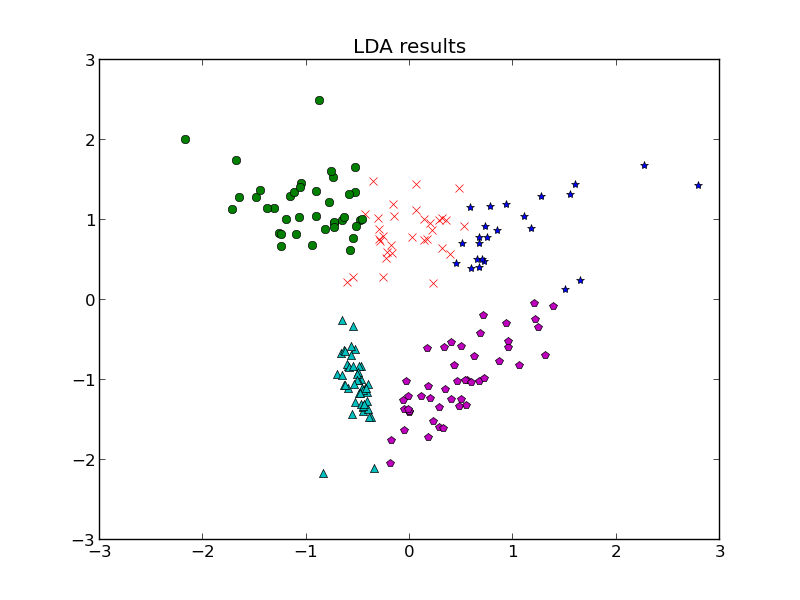
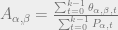
Given things: n states, m observations, A transition matrix with n rows by n columns, O transition matrix with n rows by m columns, and k observations in a vector Y with elements for each time step 1 to k. A and O can be filled with appropriate uniform probability values if we really have no idea what should go in there.

Expectation step

1. Do forward-backward algorithm to get forward probabilities and backward probabilities , where the subscripts mean state i, time step j, where F and B are both 2D arrays with n rows and k+1 columns.

2. Finish forward-backward algorithm to get the final 2D array of probabilities P with n rows and k+1 columns, where elements is the probability of being at state i at time j.

Maximization step

2. We need the probabilities of being at state at time j, and at time j+1, which we can find using the following calculation.

You can see that the formula is the probability of being at state at time j, times the transition probability from to , the probability of being at state at time j+1, and the probability of the observation happening given we’re now at state . You can store this as a 3D array or something.

3. Find the new transition matrix A by calculating each element

This can be summarized as the sum of probabilities of going from state to at each time stamp over the sum of probabilities of just being in state i (and going anywhere for the next state).

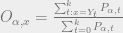
4. Find the new transition matrix B by calculating each element . This is calculating the probabilities of being in a state at the times that the observation x happened divided by the probabilities that we are in that state at any time.

5. Go back to the expectation step, and repeat until convergence.

Below, I have python code for doing the Baum-Welch algorithm. Note that I use observations similar to before, so we would expect our observation and probability matrices to not be the same as before because of my artificially manufactured observations that are stuck on a single state. Note also that above, I mentioned the solution will hit a local best solution, not necessarily what you wanted to see.

import numpy as np
# functions and classes go here
def fb_alg(A_mat, O_mat, observ):
    # set up
    k = observ.size
    (n,m) = O_mat.shape
    prob_mat = np.zeros( (n,k) )
    fw = np.zeros( (n,k+1) )
    bw = np.zeros( (n,k+1) )
    # forward part
    fw[:, 0] = 1.0/n
    for obs_ind in xrange(k):
        f_row_vec = np.matrix(fw[:,obs_ind])
        fw[:, obs_ind+1] = f_row_vec * \
                           np.matrix(A_mat) * \
                           np.matrix(np.diag(O_mat[:,observ[obs_ind]]))
        fw[:,obs_ind+1] = fw[:,obs_ind+1]/np.sum(fw[:,obs_ind+1])
    # backward part
    bw[:,-1] = 1.0
    for obs_ind in xrange(k, 0, -1):
        b_col_vec = np.matrix(bw[:,obs_ind]).transpose()
        bw[:, obs_ind-1] = (np.matrix(A_mat) * \
                            np.matrix(np.diag(O_mat[:,observ[obs_ind-1]])) * \
                            b_col_vec).transpose()
        bw[:,obs_ind-1] = bw[:,obs_ind-1]/np.sum(bw[:,obs_ind-1])
    # combine it
    prob_mat = np.array(fw)*np.array(bw)
    prob_mat = prob_mat/np.sum(prob_mat, 0)
    # get out
    return prob_mat, fw, bw

def baum_welch( num_states, num_obs, observ ):
    # allocate
    A_mat = np.ones( (num_states, num_states) )
    A_mat = A_mat / np.sum(A_mat,1)
    O_mat = np.ones( (num_states, num_obs) )
    O_mat = O_mat / np.sum(O_mat,1)
    theta = np.zeros( (num_states, num_states, observ.size) )
    while True:
        old_A = A_mat
        old_O = O_mat
        A_mat = np.ones( (num_states, num_states) )
        O_mat = np.ones( (num_states, num_obs) )
        # expectation step, forward and backward probs
        P,F,B = fb_alg( old_A, old_O, observ)
        # need to get transitional probabilities at each time step too
        for a_ind in xrange(num_states):
            for b_ind in xrange(num_states):
                for t_ind in xrange(observ.size):
                    theta[a_ind,b_ind,t_ind] = \
                    F[a_ind,t_ind] * \
                    B[b_ind,t_ind+1] * \
                    old_A[a_ind,b_ind] * \
                    old_O[b_ind, observ[t_ind]]
        # form A_mat and O_mat
        for a_ind in xrange(num_states):
            for b_ind in xrange(num_states):
                A_mat[a_ind, b_ind] = np.sum( theta[a_ind, b_ind, :] )/ \
                                      np.sum(P[a_ind,:])
        A_mat = A_mat / np.sum(A_mat,1)
        for a_ind in xrange(num_states):
            for o_ind in xrange(num_obs):
                right_obs_ind = np.array(np.where(observ == o_ind))+1
                O_mat[a_ind, o_ind] = np.sum(P[a_ind,right_obs_ind])/ \
                                      np.sum( P[a_ind,1:])
        O_mat = O_mat / np.sum(O_mat,1)
        # compare
        if np.linalg.norm(old_A-A_mat) < .00001 and np.linalg.norm(old_O-O_mat) < .00001:
            break
    # get out
    return A_mat, O_mat

num_obs = 25
observations1 = np.random.randn( num_obs )
observations1[observations1>0] = 1
observations1[observations1<=0] = 0
A_mat, O_mat = baum_welch(2,2,observations1)
print observations1
print A_mat
print O_mat
observations2 = np.random.random(num_obs)
observations2[observations2>.15] = 1
observations2[observations2<=.85] = 0
A_mat, O_mat = baum_welch(2,2,observations2)
print observations2
print A_mat
print O_mat
A_mat, O_mat = baum_welch(2,2,np.hstack( (observations1, observations2) ) )
print A_mat
print O_mat

If you run the code as I have shown up here, you’ll notice some strange behavior involving our model. Because our model is so simplistic and we have absolutely no prior data on the coin bias and the tendency to switch, we set everything to uniform probability. The algorithm for all three cases then results in the observations being a ratio based on what the observations were, which makes sense, and the transition matrix for the states remains uniform and untouched. Obviously, then the Baum Welch algorithm here basically ignores the fact that we have a hidden Markov model and goes for the maximum likelihood estimate of the coin bias and reports that this is the observation probability for both states. This isn’t wrong, but it really may not be what you wanted to see either. The only real way to solve this is by giving the system a prior that helps solve whatever we are trying to do.

This is actually less of a problem had we modeled our hidden Markov model to have multivariate Gaussian mixtures for the observation probabilities instead of discrete values, say if we were trying to observe returned samples of a population or something. But here, it’s clear we show that Baum Welch algorithm gives us a solution, but the usefulness in this gambling bit is pretty limited.

Maximum a Posteriori Estimator and Maximum Likelihood Estimator

When I learned about these estimators, I was taking something like a class on Method of Detection and Estimation, and a Digital Communications class. In the estimation class, I had absolutely no idea what the professor was talking about when these were derived, not to mention what was its use and why he likelihood function and likelihood ratio were all mixed together into a jumble of words that didn’t quite match what he probably intended. The digital communications class explained it more simply using Bayes’ rule, and that’s what I want to do. I think it’s easier to see where these two come from, and why they even remotely make sense.

Let’s say we have n samples, and we’ll call each sample , and if we need it, we can have them all in a vector, . We guess that for sample is independent, and distributed exponentially, i.e. each sample is drawn from a probability distribution with the PDF of

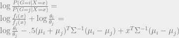
But we don’t know what actually is. Well, what can we do? We know from Bayes theorem,

We can use this to get

Our goal then is to find the value of that maximizes this expression. With a bit of calculus knowledge (i.e. finding the derivative of an expression and setting it to 0 to find critical points), we can find a parameter value that probably fits the samples we have.

But doesn’t that right side look difficult? First, since we’re maximizing over the parameter value, the bottom part of the fraction is essentially a constant that doesn’t play into our equation. And that simply leaves us with the distribution of the parameter, and the probably of getting our samples, given the parameter.

That still leaves the distribution of the parameter up for question. If we have no prior knowledge about the distribution of , then we can fill in a constant in the place of that prior distribution. Conceptually, we are claiming that the parameter is distributed uniformly in an infinitely long interval such that the PDF of the prior is just some value barely greater than 0 everywhere. With both the prior and the bottom part of the fraction constant, then we are left trying to maximize

Which awesome enough, is the maximum likelihood estimator, and the right side is known as the likelihood function. So the maximum likelihood function is basically the maximum a posteriori estimator, but we don’t have any real prior knowledge about the distribution of the parameter yet.

Thanks to the properties of logarithms, we can make the problem even simpler by finding the maximum of the log likelihood function, simply taking the log of the likelihood function and working on finding the maximum of that. The maximum point will still be the same.

Let’s do an MLE example. Say we have n samples, probably distribution exponentially, and we want to find the parameter that fits our data the best. I don’t have any prior knowledge of the distribution of the parameter, so I can’t really use MAP here. We get the following likelihood function

If we find the log of this, we get

Find the derivative w.r.t. and set it to 0 in true calculus style

We solve for the parameter, and lo and behold, we get

The sample average is our maximum likelihood estimator! I’m not going to check that this is actually a maximum by using a 2nd derivative, but it is heavily recommended that you do.