Interesting Applications of Amplitude Modulation of Signals

I had a hard time thinking about what to write, and I settling with amplitude modulation. So let’s get down to it.

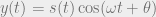
Simply put, amplitude modulation of a signal causes a signal to have sinusoidal fluctuations in amplitude. The simplest form of AM can be shown in this equation, given a signal

is some radian frequency oscillation rate, is a possible phase offset, and is obviously time.

I made a plot below that visibly shows the effects of basic amplitude modulation below on a simple triangle wave. Code is available at the bottom of the page. You can see the ENVELOPE of the signal, i.e. the original triangle wave, though it goes positive and negative thanks to the cosine wave. Additionally, in the frequency domain, you can see the fat spike of the triangle wave getting spun up to the frequency of the cosine wave! This is how basic AM radio works, the original signal is spun up to a higher carrier frequency before being transmitted over the air!

Amplitude modulation isn’t described only by the equation above, it’s a blanket term for affecting the amplitude of a signal with a sinusoidal function, so as you can imagine, different applications get different equations for different purposes.

The equation given above has a use in audio effects known as “TREMOLO.” You can buy a tremolo pedal for electric guitars, and a lot of nicer solid-state or DSP-based amplifier systems like Line6’s Spider series generally have a tremolo function built in. The most obvious use of it is in the beginning of Boulevard of Broken Dreams by Green Day, from the 2004 album American Idiot. Aside from arguments concerning musical taste, the simple chord progression makes it very clear what tremolo effects sound like.

In radio, amplitude modulation takes a huge turn into complexity land because of its various applications and uses in both analog and digital radio. The simple equation above is known as double-sideband suppressed carrier, as opposed to double-sideband AM which is like

There are other types of analog AM like single-sideband varieties. Say, single-sideband suppressed carrier with an equation like this:

The varying radio types require different receivers and have different power requirements, not to mention analog implementation of transmitters is also sort of rigid in terms of design. Modern digital communications using pulse amplitude modulation or quadrature amplitude modulation also build on the AM idea, but using a fixed constellation size and flexible parameters, they allow for much more reliable communications than analog methods in general, not to mention basic nice things you get from putting data into bits (forward error correction, etc).

I’m sure there are other useful things that amplitude modulation can do, but those are the two I’m most attuned with.

Oh yeah, the code I promised for making those plots.

# -*- coding: utf-8 -*-
"""
Created on Tue Mar 18 23:46:58 2014

@author: joshua
"""

import numpy as np
import matplotlib.pyplot as plt
# initialize a triangle wave
triangle = np.hstack( (np.zeros(15), np.linspace(0,1,50), np.linspace(1,0,50), np.zeros(15)) )
n = np.size(triangle)
# initialize a cosine wave
the_cos = np.cos(2*np.pi*.2*np.arange(n))
# multiply 
the_result = triangle*the_cos
# plot triangle
plt.figure()
plt.subplot(3,1,1)
plt.plot(np.arange(n), triangle)
plt.xlabel('sample index')
plt.ylabel('amplitude')
plt.title( 'triangle wave' )
# plot cosine
plt.subplot(3,1,2)
plt.plot(np.arange(n), the_cos)
plt.xlabel('sample index')
plt.ylabel('amplitude')
plt.title( 'carrier cosine' )
# plot both together
plt.subplot(3,1,3)
plt.plot(np.arange(n), the_result)
plt.xlabel('sample index')
plt.ylabel('amplitude')
plt.title( 'AM result' )
plt.tight_layout()
# save it
plt.savefig('am_demo_1.png')
# plot triangle FFT
plt.clf()
plt.subplot(3,1,1)
plt.plot(np.linspace(0, 2*np.pi, num=n, endpoint=False), np.abs(np.fft.fft(triangle)))
plt.xlabel('freq in radians')
plt.ylabel('magnitude')
plt.title( 'triangle wave in frequency' )
# plot cosine FFT
plt.subplot(3,1,2)
plt.plot(np.linspace(0, 2*np.pi, num=n, endpoint=False), np.abs(np.fft.fft(the_cos)))
plt.xlabel('freq in radians')
plt.ylabel('magnitude')
plt.title( 'cos in frequency' )
# plot both FFT
plt.subplot(3,1,3)
plt.plot(np.linspace(0, 2*np.pi, num=n, endpoint=False), np.abs(np.fft.fft(the_result)))
plt.xlabel('freq in radians')
plt.ylabel('magnitude')
plt.title( 'AM result in frequency' )
plt.tight_layout()
# save it
plt.savefig('am_demo_2.png')

Passband and Baseband signal representation

I think this is worth bringing up because I never covered it in any signal processing class, but I certainly went over several times in different wireless/digital communication classes at UT. I had to use this in an acoustics application at work once on somebody else’s project, and it occurred to me this may not be common knowledge (my friend certainly didn’t know about it at the time). So let’s talk about it.

So let’s say we have a band-limited passband signal, say, an ideal noiseless radio signal going from a wireless radio to some other wireless radio. We can represent any signal of this type mathematically as

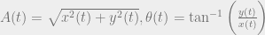
Here, the amplitude of our signal is represented by as a function of time, is the carrier frequency (in radians) that our passband signal is centered at, and is a phase component that is a function of time. So right off the bat, we can see that amplitude modulation and frequency modulation can be easily put into this form because of the general way we are expressing amplitude and phase of the signal.

We can express our passband signal in a slightly different way if we say that , and with some trigonometry identities, we can get the following representation of our signal.

With not too much imagination, you can see that

Finally, we can get our baseband representation of our signal by taking the x and y components (the inphase and quadrature parts, respectively), and getting the following.

where j is our imaginary number because I’m an electrical engineer and that’s what I’m used to using.

For the application I had at work, my friend had a baseband signal acoustic signal. Clearly it could not be played as is because it had real and imaginary parts to it, so we multiplied the real component by cosine, imaginary component (without the imaginary part) by negative sine, and we got what sounded like an underwater ping with reverberation from the ocean floor.

So why did I need to learn this for wireless communications? We know that radio signals are at some high frequency thanks to packaging materials on electronics. However, working with signals while they are at said frequency is needlessly difficulty and costly, especially when the actual bandwidth of our signal is much smaller. So we can work with a signal at baseband, spin it up to radio frequency, and receive it by spinning it down to baseband again and then decoding it. Essentially, everything we want to do, we can do it at baseband, and just spin it up to radio frequency when we’re done.