I’ve talked about Markov chains, hidden Markov models, and the Viterbi algorithm for finding the most probable path of states in a hidden Markov model. Moving on, let’s say we want to know the actual probability of each state at each time step of our process, given the observations. The algorithm to do this with is called the forward-backward algorithm.
So we have our hidden Markov model from before, transition matrix A, observation matrix O, with n states, m observations such that A is n rows by n columns, and O is n rows by m columns. Say our sequence of states that happened is X, with each time stamp denoted as 

The approximation is there because there is some scaling denominator in Bayes theorem that should be be there, but we can figure that out after the fact in our algorithm. We can see that the probability of being in state i at time j, given the observations we saw, can be broken up into two parts, one of which is the probability of a state given the observations up until that point times the probability of the observations after that point in time, given the state. We divide these up into a forward propagation step, and a backward propagation step, described using the following,

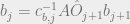
where f is a row vector of n elements containing our forward probabilities at whatever time step, and b is a column vector of n elements containing our backward probabiltiies at whatever time step, A is our transition matrix like before, and this new 
Why would we do this? Aside from it being part of the Baum-Welch algorithm, it should be pretty clear why we want to see the probability of each state at each time step. There may be cases where the best path as determined by the Viterbi algorithm or something is deemed incorrect, and it may be worth going back through the actual probability values and attempting to find where some sort of ambiguity or anomaly tripped up our dynamic programming solution.
Under the assumption we’re using MATLAB or Python, something with proper matrix and array support, the forward and backward algorithm is pretty simple. The algorithm is described in full below.
Forward propagation
1. initialize some starting row vector f at time 0 (this is where you’d want to put prior information if you have it, otherwise, just make the probability of each state 
2. For each time step, propagate forward
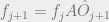
3. Normalize the resulting f vector at time j+1. Save the result somewhere, we’re gonna need it at the end.
4. Return to step 2 and keep propagating until you are out of observations.
Backward propagation
5. initialize n-element column vector of 1s as probability of being in each state at the end of the process (since the initial state of these is assumed to be given, like we already know we are ending in whatever state, the probability of ending in each of these is 1).
6. For each time step, propagate backwards

7. Normalize the resulting b vector at time j. Save this result somewhere too, we’ll need it.
8. Return to step 6 and keep propagating backwards until you are out of observations.
Putting it all together
9. Multiply all of your forwards and backwards probabilities together, matching values by states and time-steps. If you had organized your probabilities for forwards and backwards propagation into n by k matrices, you can just do an element multiply and end up with the wanted result.
10. Normalize each time step’s probabilities again. Darnit, Bayes.
So below, I have a Python implementation of the forward-backward algorithm using the fair coin biased coin example from before.
# imports go here
import numpy as np
# functions and classes go here
def fb_alg(A_mat, O_mat, observ):
    # set up
    k = observ.size
    (n,m) = O_mat.shape
    prob_mat = np.zeros( (n,k) )
    fw = np.zeros( (n,k+1) )
    bw = np.zeros( (n,k+1) )
    # forward part
    fw[:, 0] = 1.0/n
    for obs_ind in xrange(k):
        f_row_vec = np.matrix(fw[:,obs_ind])
        fw[:, obs_ind+1] = f_row_vec * \
                           np.matrix(A_mat) * \
                           np.matrix(np.diag(O_mat[:,observ[obs_ind]]))
        fw[:,obs_ind+1] = fw[:,obs_ind+1]/np.sum(fw[:,obs_ind+1])
    # backward part
    bw[:,-1] = 1.0
    for obs_ind in xrange(k, 0, -1):
        b_col_vec = np.matrix(bw[:,obs_ind]).transpose()
        bw[:, obs_ind-1] = (np.matrix(A_mat) * \
                            np.matrix(np.diag(O_mat[:,observ[obs_ind-1]])) * \
                            b_col_vec).transpose()
        bw[:,obs_ind-1] = bw[:,obs_ind-1]/np.sum(bw[:,obs_ind-1])
    # combine it
    prob_mat = np.array(fw)*np.array(bw)
    prob_mat = prob_mat/np.sum(prob_mat, 0)
    # get out
    return prob_mat, fw, bw

# main script stuff goes here
if __name__ == '__main__':
    # the transition matrix
    A_mat = np.array([[.6, .4], [.2, .8]])
    # the observation matrix
    O_mat = np.array([[.5, .5], [.15, .85]])
    # sample heads or tails, 0 is heads, 1 is tails
    num_obs = 15
    observations1 = np.random.randn( num_obs )
    observations1[observations1>0] = 1
    observations1[observations1<=0] = 0
    p,f,b = fb_alg(A_mat, O_mat, observations1)
    print p
    # change observations to reflect messed up ratio
    observations2 = np.random.random(num_obs)
    observations2[observations2>.85] = 0
    observations2[observations2<=.85] = 1
    # majority of the time its tails, now what?
    p,f,b = fb_alg(A_mat, O_mat, observations1)
    print p
    p,f,b = fb_alg(A_mat, O_mat, np.hstack( (observations1, observations2) ))
    print p
If you run the code, using the examples from the previous post, we can see that in general, for observation 1 the probabilities tend to be on the side of fair coin state, though it can sway easily. Observation 2 is definitely more on the biased coin side, and for the extended observation 3, you can see initially it is more on the fair coin state with a lot of swaying, but the latter half is almost dead on the biased coin side.
But realistically, we may not know the transition or observation matrices to our model beforehand. What’s a good way to try and estimate them? The Baum-Welch algorithm is a version of the expectation-maximization algorithm used for hidden Markov models, and it uses the forward backward algorithm for part of the process. We will talk about that next.
