Baum-Welch algorithm: Finding parameters for our HMM

Up to this point, I’ve discussed hidden Markov models, the Viterbi algorithm, and the forward-backward algorithm. This is all fun and great, but we’ve also made the assumption that we know or assume a lot of information about the HMM. In a lot of cases, we would like a way to estimate the transition matrix A and the observation matrix O, but how would we go about doing that?

The expectation-maximization algorithm can be discussed in detail later, but the Baum-Welch algorithm is considered to be an application of the EM algorithm for use with HMMs. The idea here is that we can start with some sort of prior A and O matrix, possibly a trivial one with completely uniform probabilities, and we have a set of observations from the HMM. We use the forward-backward algorithm to calculate the probabilities of being in each state at each time step, and then we use this estimate of probabilities to make a better estimate of the transition and observation matrices. Using these improved (hopefully) A and O matrices, we do forward-backwards algorithm again, and the cycle continues until the A and O matrices converge and we can call it a day.

As for why the expectation maximization idea even works, the proof isn’t trivial, you can check Wikipedia, but essentially the EM algorithm tends to converge to some local solution that is feasible for the observations and prior distributions given, but may not be the actual parameters to the problem.

So let’s break down Baum-Welch. We split it up into expectation and maximization steps just to make it a point that we have two different parts.

Given things: n states, m observations, A transition matrix with n rows by n columns, O transition matrix with n rows by m columns, and k observations in a vector Y with elements for each time step 1 to k. A and O can be filled with appropriate uniform probability values if we really have no idea what should go in there.

Expectation step

1. Do forward-backward algorithm to get forward probabilities and backward probabilities , where the subscripts mean state i, time step j, where F and B are both 2D arrays with n rows and k+1 columns.

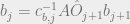
2. Finish forward-backward algorithm to get the final 2D array of probabilities P with n rows and k+1 columns, where elements is the probability of being at state i at time j.

Maximization step

2. We need the probabilities of being at state at time j, and at time j+1, which we can find using the following calculation.

You can see that the formula is the probability of being at state at time j, times the transition probability from to , the probability of being at state at time j+1, and the probability of the observation happening given we’re now at state . You can store this as a 3D array or something.

3. Find the new transition matrix A by calculating each element

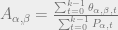
This can be summarized as the sum of probabilities of going from state to at each time stamp over the sum of probabilities of just being in state i (and going anywhere for the next state).

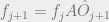
4. Find the new transition matrix B by calculating each element 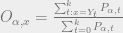. This is calculating the probabilities of being in a state at the times that the observation x happened divided by the probabilities that we are in that state at any time.

5. Go back to the expectation step, and repeat until convergence.

Below, I have python code for doing the Baum-Welch algorithm. Note that I use observations similar to before, so we would expect our observation and probability matrices to not be the same as before because of my artificially manufactured observations that are stuck on a single state. Note also that above, I mentioned the solution will hit a local best solution, not necessarily what you wanted to see.

import numpy as np
# functions and classes go here
def fb_alg(A_mat, O_mat, observ):
    # set up
    k = observ.size
    (n,m) = O_mat.shape
    prob_mat = np.zeros( (n,k) )
    fw = np.zeros( (n,k+1) )
    bw = np.zeros( (n,k+1) )
    # forward part
    fw[:, 0] = 1.0/n
    for obs_ind in xrange(k):
        f_row_vec = np.matrix(fw[:,obs_ind])
        fw[:, obs_ind+1] = f_row_vec * \
                           np.matrix(A_mat) * \
                           np.matrix(np.diag(O_mat[:,observ[obs_ind]]))
        fw[:,obs_ind+1] = fw[:,obs_ind+1]/np.sum(fw[:,obs_ind+1])
    # backward part
    bw[:,-1] = 1.0
    for obs_ind in xrange(k, 0, -1):
        b_col_vec = np.matrix(bw[:,obs_ind]).transpose()
        bw[:, obs_ind-1] = (np.matrix(A_mat) * \
                            np.matrix(np.diag(O_mat[:,observ[obs_ind-1]])) * \
                            b_col_vec).transpose()
        bw[:,obs_ind-1] = bw[:,obs_ind-1]/np.sum(bw[:,obs_ind-1])
    # combine it
    prob_mat = np.array(fw)*np.array(bw)
    prob_mat = prob_mat/np.sum(prob_mat, 0)
    # get out
    return prob_mat, fw, bw

def baum_welch( num_states, num_obs, observ ):
    # allocate
    A_mat = np.ones( (num_states, num_states) )
    A_mat = A_mat / np.sum(A_mat,1)
    O_mat = np.ones( (num_states, num_obs) )
    O_mat = O_mat / np.sum(O_mat,1)
    theta = np.zeros( (num_states, num_states, observ.size) )
    while True:
        old_A = A_mat
        old_O = O_mat
        A_mat = np.ones( (num_states, num_states) )
        O_mat = np.ones( (num_states, num_obs) )
        # expectation step, forward and backward probs
        P,F,B = fb_alg( old_A, old_O, observ)
        # need to get transitional probabilities at each time step too
        for a_ind in xrange(num_states):
            for b_ind in xrange(num_states):
                for t_ind in xrange(observ.size):
                    theta[a_ind,b_ind,t_ind] = \
                    F[a_ind,t_ind] * \
                    B[b_ind,t_ind+1] * \
                    old_A[a_ind,b_ind] * \
                    old_O[b_ind, observ[t_ind]]
        # form A_mat and O_mat
        for a_ind in xrange(num_states):
            for b_ind in xrange(num_states):
                A_mat[a_ind, b_ind] = np.sum( theta[a_ind, b_ind, :] )/ \
                                      np.sum(P[a_ind,:])
        A_mat = A_mat / np.sum(A_mat,1)
        for a_ind in xrange(num_states):
            for o_ind in xrange(num_obs):
                right_obs_ind = np.array(np.where(observ == o_ind))+1
                O_mat[a_ind, o_ind] = np.sum(P[a_ind,right_obs_ind])/ \
                                      np.sum( P[a_ind,1:])
        O_mat = O_mat / np.sum(O_mat,1)
        # compare
        if np.linalg.norm(old_A-A_mat) < .00001 and np.linalg.norm(old_O-O_mat) < .00001:
            break
    # get out
    return A_mat, O_mat

num_obs = 25
observations1 = np.random.randn( num_obs )
observations1[observations1>0] = 1
observations1[observations1<=0] = 0
A_mat, O_mat = baum_welch(2,2,observations1)
print observations1
print A_mat
print O_mat
observations2 = np.random.random(num_obs)
observations2[observations2>.15] = 1
observations2[observations2<=.85] = 0
A_mat, O_mat = baum_welch(2,2,observations2)
print observations2
print A_mat
print O_mat
A_mat, O_mat = baum_welch(2,2,np.hstack( (observations1, observations2) ) )
print A_mat
print O_mat

If you run the code as I have shown up here, you’ll notice some strange behavior involving our model. Because our model is so simplistic and we have absolutely no prior data on the coin bias and the tendency to switch, we set everything to uniform probability. The algorithm for all three cases then results in the observations being a ratio based on what the observations were, which makes sense, and the transition matrix for the states remains uniform and untouched. Obviously, then the Baum Welch algorithm here basically ignores the fact that we have a hidden Markov model and goes for the maximum likelihood estimate of the coin bias and reports that this is the observation probability for both states. This isn’t wrong, but it really may not be what you wanted to see either. The only real way to solve this is by giving the system a prior that helps solve whatever we are trying to do.

This is actually less of a problem had we modeled our hidden Markov model to have multivariate Gaussian mixtures for the observation probabilities instead of discrete values, say if we were trying to observe returned samples of a population or something. But here, it’s clear we show that Baum Welch algorithm gives us a solution, but the usefulness in this gambling bit is pretty limited.

Forward-backward Algorithm: Finding probability of states at each time step in an HMM

I’ve talked about Markov chains, hidden Markov models, and the Viterbi algorithm for finding the most probable path of states in a hidden Markov model. Moving on, let’s say we want to know the actual probability of each state at each time step of our process, given the observations. The algorithm to do this with is called the forward-backward algorithm.

So we have our hidden Markov model from before, transition matrix A, observation matrix O, with n states, m observations such that A is n rows by n columns, and O is n rows by m columns. Say our sequence of states that happened is X, with each time stamp denoted as , where k is the number of time steps that we are dealing with. We have a set of observations Y, also a vector k long, that we saw happen, and we want to know the probabilities of each state at each time step. By the magic of Bayes theorem, we can express our probability of a being in state i at time j, given all of our k observations, to be

The approximation is there because there is some scaling denominator in Bayes theorem that should be be there, but we can figure that out after the fact in our algorithm. We can see that the probability of being in state i at time j, given the observations we saw, can be broken up into two parts, one of which is the probability of a state given the observations up until that point times the probability of the observations after that point in time, given the state. We divide these up into a forward propagation step, and a backward propagation step, described using the following,

where f is a row vector of n elements containing our forward probabilities at whatever time step, and b is a column vector of n elements containing our backward probabiltiies at whatever time step, A is our transition matrix like before, and this new is a diagonal matrix that contains the probabilities of seeing the observation that we did for each of the states on the corresponding diagonal element. As mentioned before, we left out some scaling factor in our Bayes theorem, so we need to make sure at each time step, the probabilities of being in each state sum to 1. We can just sum the vector get at each time step and just divide the vector by the sum.

Why would we do this? Aside from it being part of the Baum-Welch algorithm, it should be pretty clear why we want to see the probability of each state at each time step. There may be cases where the best path as determined by the Viterbi algorithm or something is deemed incorrect, and it may be worth going back through the actual probability values and attempting to find where some sort of ambiguity or anomaly tripped up our dynamic programming solution.

Under the assumption we’re using MATLAB or Python, something with proper matrix and array support, the forward and backward algorithm is pretty simple. The algorithm is described in full below.

Forward propagation

1. initialize some starting row vector f at time 0 (this is where you’d want to put prior information if you have it, otherwise, just make the probability of each state .

2. For each time step, propagate forward 

3. Normalize the resulting f vector at time j+1. Save the result somewhere, we’re gonna need it at the end.

4. Return to step 2 and keep propagating until you are out of observations.

Backward propagation

5. initialize n-element column vector of 1s as probability of being in each state at the end of the process (since the initial state of these is assumed to be given, like we already know we are ending in whatever state, the probability of ending in each of these is 1).

6. For each time step, propagate backwards 

7. Normalize the resulting b vector at time j. Save this result somewhere too, we’ll need it.

8. Return to step 6 and keep propagating backwards until you are out of observations.

Putting it all together

9. Multiply all of your forwards and backwards probabilities together, matching values by states and time-steps. If you had organized your probabilities for forwards and backwards propagation into n by k matrices, you can just do an element multiply and end up with the wanted result.

10. Normalize each time step’s probabilities again. Darnit, Bayes.

So below, I have a Python implementation of the forward-backward algorithm using the fair coin biased coin example from before.

# imports go here
import numpy as np
# functions and classes go here
def fb_alg(A_mat, O_mat, observ):
    # set up
    k = observ.size
    (n,m) = O_mat.shape
    prob_mat = np.zeros( (n,k) )
    fw = np.zeros( (n,k+1) )
    bw = np.zeros( (n,k+1) )
    # forward part
    fw[:, 0] = 1.0/n
    for obs_ind in xrange(k):
        f_row_vec = np.matrix(fw[:,obs_ind])
        fw[:, obs_ind+1] = f_row_vec * \
                           np.matrix(A_mat) * \
                           np.matrix(np.diag(O_mat[:,observ[obs_ind]]))
        fw[:,obs_ind+1] = fw[:,obs_ind+1]/np.sum(fw[:,obs_ind+1])
    # backward part
    bw[:,-1] = 1.0
    for obs_ind in xrange(k, 0, -1):
        b_col_vec = np.matrix(bw[:,obs_ind]).transpose()
        bw[:, obs_ind-1] = (np.matrix(A_mat) * \
                            np.matrix(np.diag(O_mat[:,observ[obs_ind-1]])) * \
                            b_col_vec).transpose()
        bw[:,obs_ind-1] = bw[:,obs_ind-1]/np.sum(bw[:,obs_ind-1])
    # combine it
    prob_mat = np.array(fw)*np.array(bw)
    prob_mat = prob_mat/np.sum(prob_mat, 0)
    # get out
    return prob_mat, fw, bw

# main script stuff goes here
if __name__ == '__main__':
    # the transition matrix
    A_mat = np.array([[.6, .4], [.2, .8]])
    # the observation matrix
    O_mat = np.array([[.5, .5], [.15, .85]])
    # sample heads or tails, 0 is heads, 1 is tails
    num_obs = 15
    observations1 = np.random.randn( num_obs )
    observations1[observations1>0] = 1
    observations1[observations1<=0] = 0
    p,f,b = fb_alg(A_mat, O_mat, observations1)
    print p
    # change observations to reflect messed up ratio
    observations2 = np.random.random(num_obs)
    observations2[observations2>.85] = 0
    observations2[observations2<=.85] = 1
    # majority of the time its tails, now what?
    p,f,b = fb_alg(A_mat, O_mat, observations1)
    print p
    p,f,b = fb_alg(A_mat, O_mat, np.hstack( (observations1, observations2) ))
    print p

If you run the code, using the examples from the previous post, we can see that in general, for observation 1 the probabilities tend to be on the side of fair coin state, though it can sway easily. Observation 2 is definitely more on the biased coin side, and for the extended observation 3, you can see initially it is more on the fair coin state with a lot of swaying, but the latter half is almost dead on the biased coin side.

But realistically, we may not know the transition or observation matrices to our model beforehand. What’s a good way to try and estimate them? The Baum-Welch algorithm is a version of the expectation-maximization algorithm used for hidden Markov models, and it uses the forward backward algorithm for part of the process. We will talk about that next.