Let’s talk about another application of least-squares in statistical learning applications. Say we have some data, and we want to separate them into groups. We have some data that we separate into training and validation sets that we know what groups they should be in. For data in an n-dimensional space (say, the data is defined by n coordinates, or in even simpler terms, has n features), we need to find hyperplanes of dimension n-1 that will SPLIT the space in half, where everything on one side is in one group, and everything on the other side of the hyperplane is in another (Intuitively, for our purposes, you can see 2D Euclidean space can be separated into two parts by a line, which is a 1 dimensional object, and a 3D euclidean space can be split by a plane, which is a 2D object).
So how do we find said hyperplane to divide up our space? The simplest way, and probably the most common way still just because it’s easy for a first-shot attempt at classification and linear regression, is to employ least-squares.
Let us say we have 


So let’s arrange the problem thusly; we want our 
So we have our rows of data points stacked on top of each other, with a column of 1s representing a constant offset of b in our hyperplane equation. The b vector is obviously then just going to be a stack of -1s and 1s for whatever class each row data point is matched to.
And then obviously since this is least squares, our resulting 
We have our hyperplane, now how do we do validation or classification of new data points? Recall that we classified our points using -1 and 1 teams. Adding a 1 to the tail of each data point like we did before to represent the constant b term in the hyperplane equation which we have in our coefficients, we can use our hyperplane equation’s left side, 
The MATLAB code below provides an example of a hyperplane separating two 2D Gaussian populations, and then trying to use that rule to classify data with a higher variance than we expected. A plot with training data points and the separating hyperplane is generated, and then a print out of percentage of correctly classified points is given at the end.
% generate 2 2D pops
ndim = 2;
pop_size = 20;
u1 = [4, 4];
u2 = [-2, -1];
covar_mat = 5.*eye(2);
pop1 = bsxfun( @plus, randn(pop_size, ndim)*chol(covar_mat), u1 );
pop2 = bsxfun( @plus, randn(pop_size, ndim)*chol(covar_mat), u2 );
figure;
plot( pop1(:,1), pop1(:,2), '*b' );
hold on;
plot( pop2(:,1), pop2(:,2), 'xr' );
% find the hyperplane that goes through the middle using least squares
A = [[pop1; pop2], ones(2*pop_size,1)];
b = [-1.*ones( pop_size, 1 ); 1.*ones(pop_size,1)];
coefs = lscov(A, b);
% plot the coefficient line using that learning data we generated
line_x = [-20; 20];
line_y =  (-coefs(end)-coefs(1).*line_x)./coefs(2);
plot( line_x, line_y, '-k' );
xlim( [-20, 20] );
ylim( [-20, 20] );
% now let's try to classify the new points we generate
covar_mat2 = 8.*eye(2);
new_pop1 = bsxfun( @plus, randn(pop_size, ndim)*chol(covar_mat2), u1 );
new_pop2 = bsxfun( @plus, randn(pop_size, ndim)*chol(covar_mat2), u2 );
combined_newpop = [new_pop1; new_pop2];
new_inds = randperm( (2*pop_size) );
actual_population = b(new_inds);
combined_newpop = combined_newpop( new_inds, : );
newpop_w_ones = [combined_newpop, ones(2*pop_size, 1)];
classify = sum( bsxfun( @times, newpop_w_ones, coefs(:)' ), 2);
classify(classify < 0) = -1;
classify(classify >= 0) = 1;
percent_correct = sum(classify == actual_population)./(2*pop_size)
So what’s wrong with this? The clearest problem is that this method really implies that groups are linearly separable, and a lot of times, it’s not that simple. This method also tends to allow outliers to have really heavy effects on the resulting lines, and generally does poorly for classification of more than 2 groups, no matter how you decide to handle the multiple group problem (1v1 hyperplanes or 1 vs everybody else hyperplanes, either way). Inherently, since linear least squares is optimal ML estimator for Gaussian populations, you are inherently assuming multivariable Gaussian distributed stuff, and even if it is, there’s somewhat of a disregard for prior information, say, covariance matrices or anything else that might help.
Since the follow up is natural and I really want to get this stuff nailed down for myself, next time we will talk about linear discriminant analysis, and then after that, quadratic discriminant analysis. I personally think of LDA and QDA as a more thorough treatment of the linear classification problem by stating assumption and taking in account parameters that may help us, plus QDA has the benefit of generating quadratic lines.
![x[n]](https://s0.wp.com/latex.php?latex=x%5Bn%5D&bg=eeeeee&fg=666666&s=0&c=20201002) with a baseband representation at the received end like
with a baseband representation at the received end like![y[n] = x[n] \exp (j2 \pi f_{o} n T_{s} )](https://s0.wp.com/latex.php?latex=y%5Bn%5D+%3D+x%5Bn%5D+%5Cexp+%28j2+%5Cpi+f_%7Bo%7D+n+T_%7Bs%7D+%29&bg=eeeeee&fg=666666&s=0&c=20201002)
 is the frequency offset and
  is the sampling period. Looks pretty harmless, right? But wait, remember for any sort of QAM, M-PSK signaling, we require knowledge of the phase. We can’t afford to lose that, so you can imagine that the samples as you go down in sample index time start having serious phase changes from the exponential bit in the equation above. In effect, we rotate our symbols some amount of phase, and that completely messes everything up.
![t[n] \exp (j2 \pi f_{o} n T_{s} )= t[n+N_{t}] \exp( j2 \pi f_{o} (n+N_{t}) T_{s} )](https://s0.wp.com/latex.php?latex=t%5Bn%5D+%5Cexp+%28j2+%5Cpi+f_%7Bo%7D+n+T_%7Bs%7D+%29%3D+t%5Bn%2BN_%7Bt%7D%5D+%5Cexp%28+j2+%5Cpi+f_%7Bo%7D+%28n%2BN_%7Bt%7D%29+T_%7Bs%7D+%29&bg=eeeeee&fg=666666&s=0&c=20201002)
 amount of phase change between the two sequences. Well, that’s cool, that’s constant in n. We can set up a sort of trivial least-squares problem then…
![\begin{bmatrix} t[n] \\ t[n+1] \\ \vdots \\ t[n+N_{t}-1] \end{bmatrix} x = \begin{bmatrix} t[n+N_{t}] \\ t[n+N_{t}+1] \\ \vdots \\ t[n+2N_{t}-1] \end{bmatrix}](https://s0.wp.com/latex.php?latex=%5Cbegin%7Bbmatrix%7D+t%5Bn%5D+%5C%5C+t%5Bn%2B1%5D+%5C%5C+%5Cvdots+%5C%5C+t%5Bn%2BN_%7Bt%7D-1%5D+%5Cend%7Bbmatrix%7D+x+%3D+%5Cbegin%7Bbmatrix%7D+t%5Bn%2BN_%7Bt%7D%5D+%5C%5C+t%5Bn%2BN_%7Bt%7D%2B1%5D+%5C%5C+%5Cvdots+%5C%5C+t%5Bn%2B2N_%7Bt%7D-1%5D+%5Cend%7Bbmatrix%7D&bg=eeeeee&fg=666666&s=0&c=20201002)
 , and we can solve for
  .
. , so if we use too many training samples, we can’t recover a strong frequency offset.
![y[n] = \sum_{l=0}^{L} h[l] x[n-l] + v[n]](https://s0.wp.com/latex.php?latex=y%5Bn%5D+%3D+%5Csum_%7Bl%3D0%7D%5E%7BL%7D+h%5Bl%5D+x%5Bn-l%5D+%2B+v%5Bn%5D&bg=eeeeee&fg=666666&s=0&c=20201002) , where h is our discretized channel, x is the sent signal, and v is additive white Gaussian noise.
, where h is our discretized channel, x is the sent signal, and v is additive white Gaussian noise.

![\begin{bmatrix} y[L] \\ y[L+1] \\ \vdots \\ y[N_{t}-1] \end{bmatrix} = \begin{bmatrix} t[L] & \hdots & t[0] \\ t[L+1] & \ddots & \vdots \\ \vdots & & \vdots \\ t[N_{t}-1] & \hdots & t[N_{t}-1-L] \end{bmatrix} \begin{bmatrix} a[0] \\ a[1] \\ \vdots \\ a[L] \end{bmatrix}](https://s0.wp.com/latex.php?latex=%5Cbegin%7Bbmatrix%7D+y%5BL%5D+%5C%5C+y%5BL%2B1%5D+%5C%5C+%5Cvdots+%5C%5C+y%5BN_%7Bt%7D-1%5D+%5Cend%7Bbmatrix%7D+%3D+%5Cbegin%7Bbmatrix%7D+t%5BL%5D+%26+%5Chdots+%26+t%5B0%5D+%5C%5C+t%5BL%2B1%5D+%26+%5Cddots+%26+%5Cvdots+%5C%5C+%5Cvdots+%26+%26+%5Cvdots+%5C%5C+t%5BN_%7Bt%7D-1%5D+%26+%5Chdots+%26+t%5BN_%7Bt%7D-1-L%5D+%5Cend%7Bbmatrix%7D+%5Cbegin%7Bbmatrix%7D+a%5B0%5D+%5C%5C+a%5B1%5D+%5C%5C+%5Cvdots+%5C%5C+a%5BL%5D+%5Cend%7Bbmatrix%7D&bg=eeeeee&fg=666666&s=0&c=20201002)
![f[n]](https://s0.wp.com/latex.php?latex=f%5Bn%5D&bg=eeeeee&fg=666666&s=0&c=20201002) such that
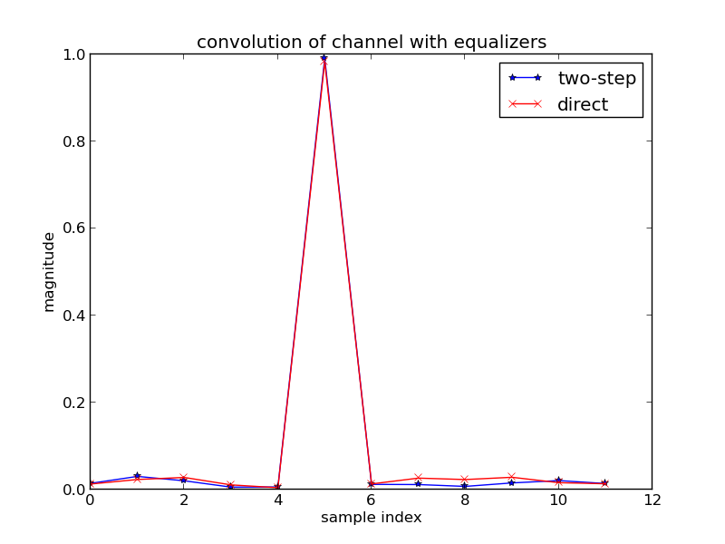
such that is the length of the equalizer filter we’re making. So we can see we want our filter to cancel out the effects of the channel and give us a Kronecker delta as a result. Realistically, we probably can’t find a great filter that will give us the delta with no time delay, so we can change our criteria such that we solve for, assuming we choose k samples worth of delay time.
![\sum_{l=0}^{L_{f}} h[l] f[n-l] = \delta[n-k]](https://s0.wp.com/latex.php?latex=%5Csum_%7Bl%3D0%7D%5E%7BL_%7Bf%7D%7D+h%5Bl%5D+f%5Bn-l%5D+%3D+%5Cdelta%5Bn-k%5D&bg=eeeeee&fg=666666&s=0&c=20201002)
![\begin{bmatrix} h[0] & 0 & \hdots & \hdots \\ h[1] & h[0] & 0 & \hdots \\ \vdots & \ddots & & \\ h[L] & & & \\ 0 & h[L] & \hdots & \\ \vdots & & & \end{bmatrix} \begin{bmatrix} f[0] \\ f[1] \\ \vdots \\ \vdots \\ \vdots \\ f[L_{f}] \end{bmatrix} = \begin{bmatrix} 0 \\ \vdots \\ 1 \\ \vdots \\ \vdots \\ 0 \end{bmatrix}](https://s0.wp.com/latex.php?latex=%5Cbegin%7Bbmatrix%7D+h%5B0%5D+%26+0+%26+%5Chdots+%26+%5Chdots+%5C%5C+h%5B1%5D+%26+h%5B0%5D+%26+0+%26+%5Chdots+%5C%5C+%5Cvdots+%26+%5Cddots+%26+%26+%5C%5C+h%5BL%5D+%26+%26+%26+%5C%5C+0+%26+h%5BL%5D+%26+%5Chdots+%26+%5C%5C+%5Cvdots+%26+%26+%26+%5Cend%7Bbmatrix%7D+%5Cbegin%7Bbmatrix%7D+f%5B0%5D+%5C%5C+f%5B1%5D+%5C%5C+%5Cvdots+%5C%5C+%5Cvdots+%5C%5C+%5Cvdots+%5C%5C+f%5BL_%7Bf%7D%5D+%5Cend%7Bbmatrix%7D+%3D+%5Cbegin%7Bbmatrix%7D+0+%5C%5C+%5Cvdots+%5C%5C+1+%5C%5C+%5Cvdots+%5C%5C+%5Cvdots+%5C%5C+0+%5Cend%7Bbmatrix%7D&bg=eeeeee&fg=666666&s=0&c=20201002)
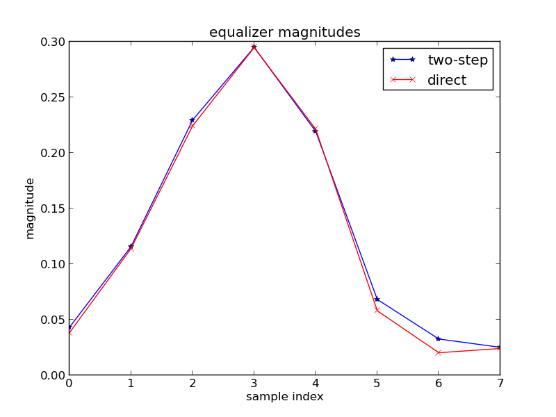
![\sum_{l=0}^{L_{f}} f[l] y[n-l] = t[n-k]](https://s0.wp.com/latex.php?latex=%5Csum_%7Bl%3D0%7D%5E%7BL_%7Bf%7D%7D+f%5Bl%5D+y%5Bn-l%5D+%3D+t%5Bn-k%5D&bg=eeeeee&fg=666666&s=0&c=20201002)
![\begin{bmatrix} t[0] \\ t[1] \\ \vdots \\ t[N_{t}-1] \end{bmatrix} = \begin{bmatrix} y[k] & \hdots & y[k-L_{f}] \\ y[k+1] & \ddots & \vdots \\ \vdots & & \vdots \\ y[k+N_{t}-1] & \hdots & y[k+N_{t}-L_{f}] \end{bmatrix} \begin{bmatrix} f[0] \\ f[1] \\ \vdots \\ f[L_{f}] \end{bmatrix}](https://s0.wp.com/latex.php?latex=%5Cbegin%7Bbmatrix%7D+t%5B0%5D+%5C%5C+t%5B1%5D+%5C%5C+%5Cvdots+%5C%5C+t%5BN_%7Bt%7D-1%5D+%5Cend%7Bbmatrix%7D+%3D+%5Cbegin%7Bbmatrix%7D+y%5Bk%5D+%26+%5Chdots+%26+y%5Bk-L_%7Bf%7D%5D+%5C%5C+y%5Bk%2B1%5D+%26+%5Cddots+%26+%5Cvdots+%5C%5C+%5Cvdots+%26+%26+%5Cvdots+%5C%5C+y%5Bk%2BN_%7Bt%7D-1%5D+%26+%5Chdots+%26+y%5Bk%2BN_%7Bt%7D-L_%7Bf%7D%5D+%5Cend%7Bbmatrix%7D+%5Cbegin%7Bbmatrix%7D+f%5B0%5D+%5C%5C+f%5B1%5D+%5C%5C+%5Cvdots+%5C%5C+f%5BL_%7Bf%7D%5D+%5Cend%7Bbmatrix%7D&bg=eeeeee&fg=666666&s=0&c=20201002)
 , gives pretty decent results.
 , and we can place them in a column vector
  for convenience. We know our polynomial is going to have some order n-1, such that our polynomial is of the form
  , so we have a total of n coefficients to our polynomial. Let’s set up the coefficients in a column vector
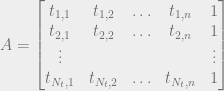
  where the T is simply a transpose, NOT a Hermitian transpose or anything. Then, we can set up our matrix X like the following.

 to
to  !
!
 discussed previously is essentially solving
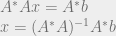
 , where Q is an m x n matrix with orthonormal columns, and R an n x n square matrix upper diagonal matrix (meaning anything below the diagonal elements are zeros), we can rewrite the least squares problem like this.
 , where U is an m x n matrix with orthonormal columns, S is a square matrix with non-negative diagonal entries, and zeroes everywhere else, and V is an n x n unitary matrix, we can turn the least squares problem into the following.
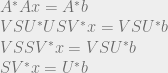

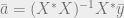
 , or A is a tall matrix. We call A an overdetermined matrix. Simply put, there are way too many unique linear equations to solve for a unique x vector answer. So what do we do? We can use least-squares formulation of the problem to get some sort of an acceptable answer. If we multiply by sides of the equation by the Hermitian transpose of A, we get
 , or A is a fat matrix, A is then an underdetermined matrix, and we have a large solution space. The vector x could be a whole number of things! What’s neat about least squares is that we can still use it here for a similar purpose.
 is minimized. There are places in optimization or control theory where we want the minimum energy vectors for controllability or stability, so the underdetermined least-squares problem is useful as well.